
XC7Z100-ADRV9009 User Manual
Set up the XC7Z100-ADRV9009 SDR platform, verify ADRV9009 connectivity, run GNU Radio modulation experiments, and inspect RF signals with IIO Oscilloscope.

Overview
This guide is organized into the following six chapters:
Product Introduction
7100-ADRV9009 Specifications and System Architecture
SD Card Firmware Programming and LibIIO Setup
Board Startup and IIO Status Verification
Installing and Using GNU Radio
IIO Oscilloscope Testing
Product Introduction
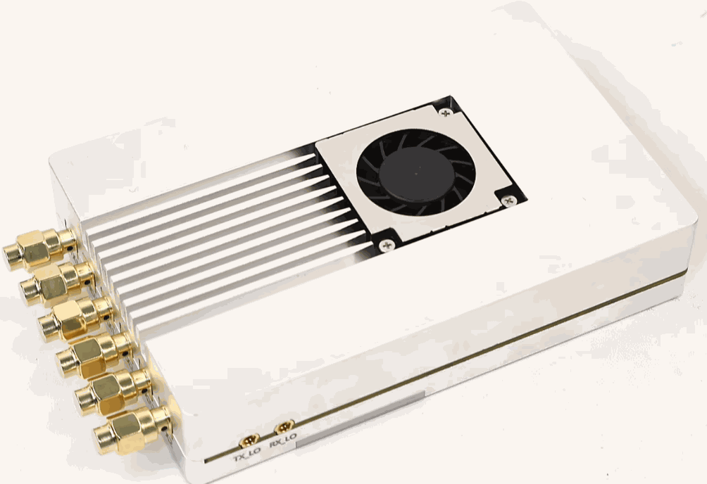
OpenSourceSDRLab's 7100-ADRV9009 is a high-performance software-defined radio (SDR) development platform built around the Xilinx Zynq-7000 XC7Z100 SoC and the Analog Devices ADRV9009 RF transceiver. Designed for SDR development, education, research, and wireless communications experiments, the platform combines embedded processing with FPGA-based signal processing.
The ADRV9009 has a nominal tuning range of 75 MHz to 6 GHz and a chip-level receive bandwidth of up to 200 MHz. The XC7Z100 integrates an ARM Cortex-A9 processing system (PS) and programmable logic (PL) in a single device, supporting embedded Linux, FPGA development, and high-speed data processing. This open-source project provides hardware documentation, a PetaLinux project, bare-metal drivers, and lwIP resources as a foundation for system development and experimentation.
7100-ADRV9009 Specifications and System Architecture
Key Specifications
Functional Block Diagram
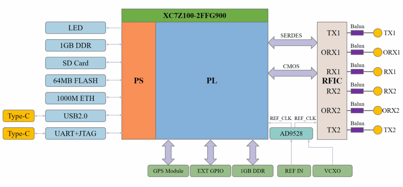
This block diagram illustrates the SDR hardware architecture built around the XC7Z100-2FFG900 Zynq SoC. The Zynq chip is internally divided into the PS (Processing System, orange section) and PL (Programmable Logic, blue section):
1.PS (ARM processor subsystem): Its peripherals include status LEDs, 1 GB DDR, SD card, 64 MB Flash, Gigabit Ethernet, USB 2.0, and one Type‑C debug port multiplexed for UART and JTAG.
2.PL (FPGA logic fabric): Connected externally to a GPS module, extended LVDS GPIO, 1 GB DDR, external reference clock input and VCXO. The PL also acts as the data bridge for the RF front end.
3.Clock unit AD9528: Generates reference clocks for the RFIC.
4.RF front-end RFIC: Consists of TX1/TX2 transmit channels, RX1/RX2 receive channels, and ORX1/ORX2 observation receive channels:
TX1 and ORX1 interface with the PL via high-speed SERDES;
RX1, RX2, ORX2 and TX2 use CMOS parallel interfaces;
Each RF signal passes through a balun and is converted to single-ended signal for the RF port.
SD Card Firmware Programming and LibIIO Setup
Writing the SD Card Image and Configuring Board Boot
1. Format the target SD card. Right-click imageUSB.exe and choose Run as administrator. In the device list, select only the SD card to be programmed to avoid overwriting another storage device.
2. Select [Write image to USB drive] as the programming option. Image path: 7100_ADRV9009资料\SD卡镜像\ADRV9009_XC7Z100.img
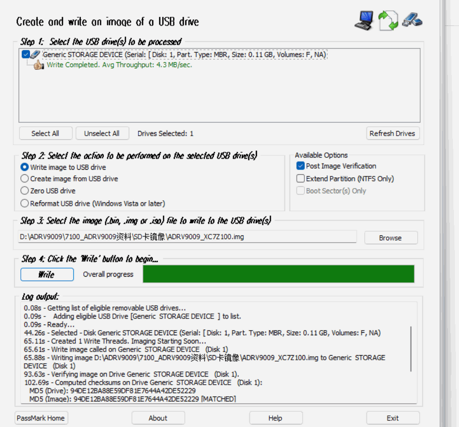
3. Confirm that the correct device is selected, then start programming. Wait for the write operation and the tool's built-in verification to finish, and safely eject the SD card.
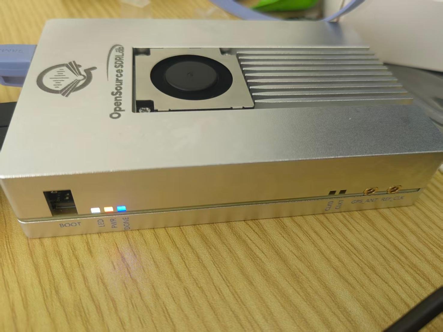
4. With the board powered off, insert the SD card and set the boot switches to SD-card boot mode. Power on the board to boot the firmware from the SD card.
Static IP Configuration
Connect the 7100-ADRV9009 directly to the computer with an Ethernet cable. Press Win+R, enter ncpa.cpl, and press Enter to open Network Connections. Right-click the active Ethernet adapter and open Properties. Double-click Internet Protocol Version 4 (TCP/IPv4), select manual IP configuration, and enter the following values:
IP address: 192.168.1.20
Subnet mask: 255.255.255.0
Default gateway: leave blank
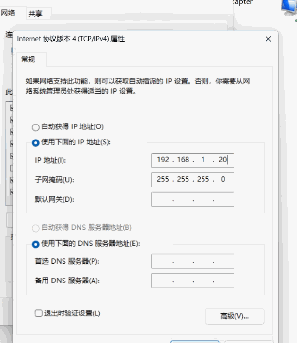
Confirm the dialogs and save the settings. The computer's static IP configuration is complete.
LibIIO Setup and Connectivity Verification
LibIIO is the core communication library used by higher-level SDR applications to interact with the 7100-ADRV9009. The Windows installer includes the required DLLs, command-line tools, and the IIO Oscilloscope graphical tool.
Choose either of the following ways to obtain the installer:
Bundled resources: Open the Windows system driver file folder. The installer is libiio-0.26.ga0eca0d2-setup.exe.
https://github.com/analogdevicesinc/libiio/releases
Installation steps:
Run libiio-0.26.ga0eca0d2-setup.exe, select a language, accept the license agreement, and complete the installation.
Open Command Prompt and run the discovery command:
iio_info -u ip:192.168.1.10
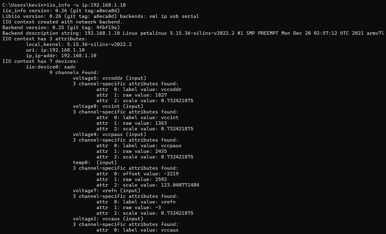
Pass criterion: If the terminal displays complete device information for the ADRV9009 transceiver, communication between the host and the board is working.
Next, verify that the ADRV9009 devices are enumerated by running this command in Command Prompt:
iio_info -u ip:192.168.1.10 | findstr /i "adrv9009 axi-adrv"

Verification criterion: If the output lists adrv9009-phy and the RX, TX, and ORX data devices, the ADRV9009 has been recognized correctly.
Board Startup and IIO Status Verification
Hardware Connections and Power-On Preparation
Insert the SD card and connect the power cable to power on the device. Check whether the PWR and DONE LEDs are steady on. Connect the USB and DEBUG cables only after both LEDs stay on.
Logging In and Collecting System Status
Open PuTTY and log in to the system, then run the following commands to record system status:
uname -a
cat /etc/petalinux/version
dmesg | grep -Ei 'adrv9009|talise|jesd|iio|firmware'
ls -l /sys/bus/iio/devices/
command -v iio_info
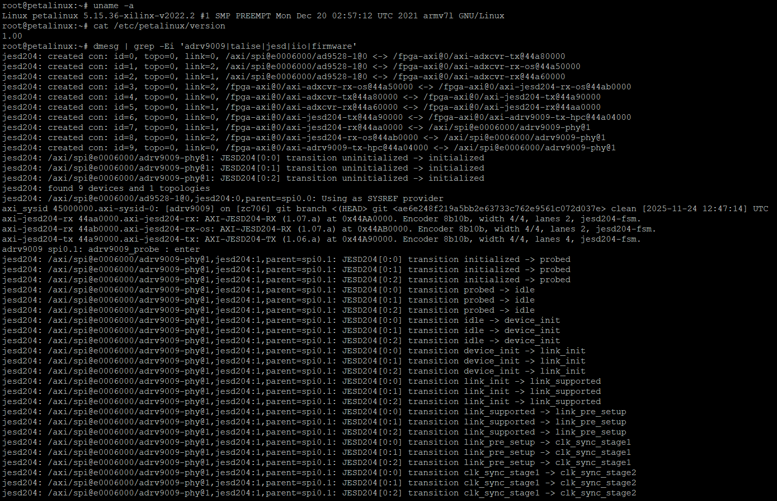
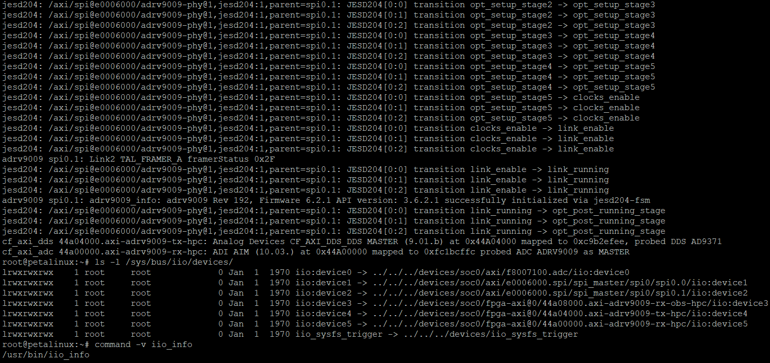
Pass criterion: The dmesg log shows the JESD204 state machine reaching link_running and prints adrv9009 successfully initialized. IIO device nodes are present under /sys/bus/iio/devices/, and the iio_info utility runs successfully. This indicates that the RF chip and IIO driver have loaded.
Installing and Using GNU Radio
GNU Radio is a powerful open-source signal-processing framework widely used for software-defined radio (SDR) development. With the GNU Radio Companion (GRC) graphical tool, users can build complex wireless communication systems without writing code.
Installing GNU Radio
Locate radioconda-2025.03.14-Windows-x86_64.exe in the software package and double-click it to launch the installer.
Capturing the ADRV9009 RX1 Baseband Spectrum with GNU Radio
Before the experiment, connect an antenna to the RX1 port, then run this command in a terminal: iio_info -s

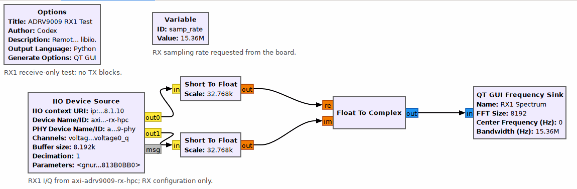
IIO Source connects to the ADRV9009 over the network and reads the RX1 voltage0_i and voltage0_q sample streams. Each stream passes through Short To Float and is normalized by 32768. Float To Complex then combines them into a complex I/Q signal, which is sent to QT GUI Frequency Sink for spectrum analysis and display.
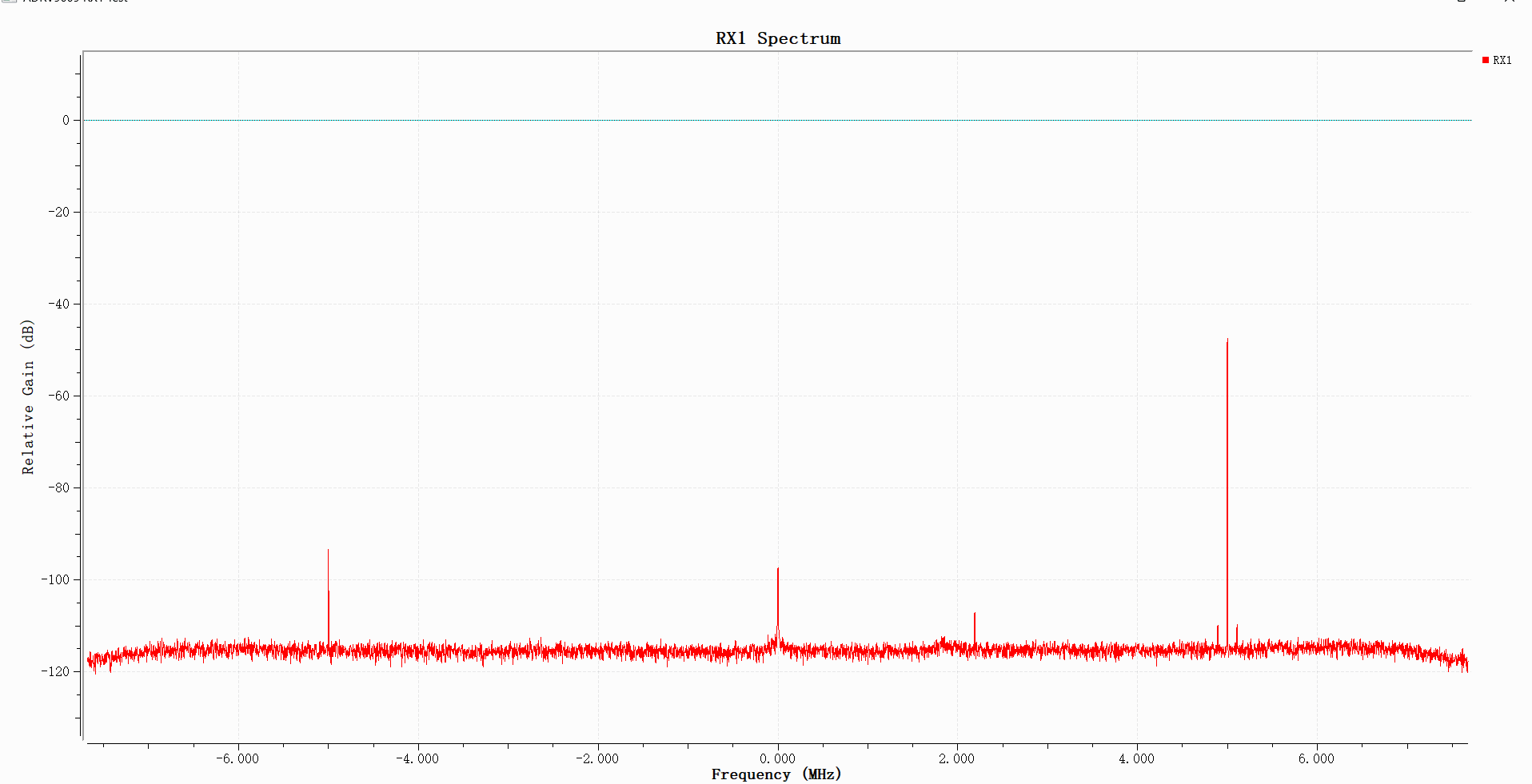
The RX1 receiver is acquiring and outputting I/Q data. The spectrum shows a continuous noise floor of about -115 dB across the receive bandwidth of approximately -7.68 to +7.68 MHz. A prominent peak appears near +5 MHz, with weaker peaks near 0 MHz and -5 MHz. This indicates that the receive chain has captured signal components.
Preparing GNU Radio Modulation Experiments
AM Modulation and Envelope Detection
Software Simulation of AM Modulation
1. Open AM_dsb_tc.grc and run the AM modulation simulation. The flowgraph uses a 50 kHz cosine wave with amplitude 1 as the simulated carrier and a 1 kHz cosine wave with amplitude 0.7 and DC offset 1 as the modulating signal. The two signals are multiplied to vary the carrier amplitude and generate an AM signal. Throttle controls the software simulation rate. QT GUI Time Sink and QT GUI Frequency Sink display the time-domain waveform and spectrum, respectively. The DC-offset modulating signal is also connected directly to a time-domain display so it can be compared with the envelope of the modulated signal.
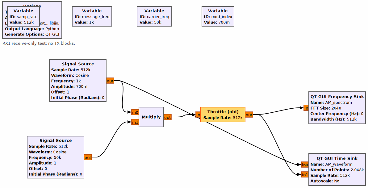
2. After running the simulation, the AM signal's spectrum and time-domain waveform are displayed. The upper half of the window shows the frequency-domain plot; the lower half shows the time-domain plot.
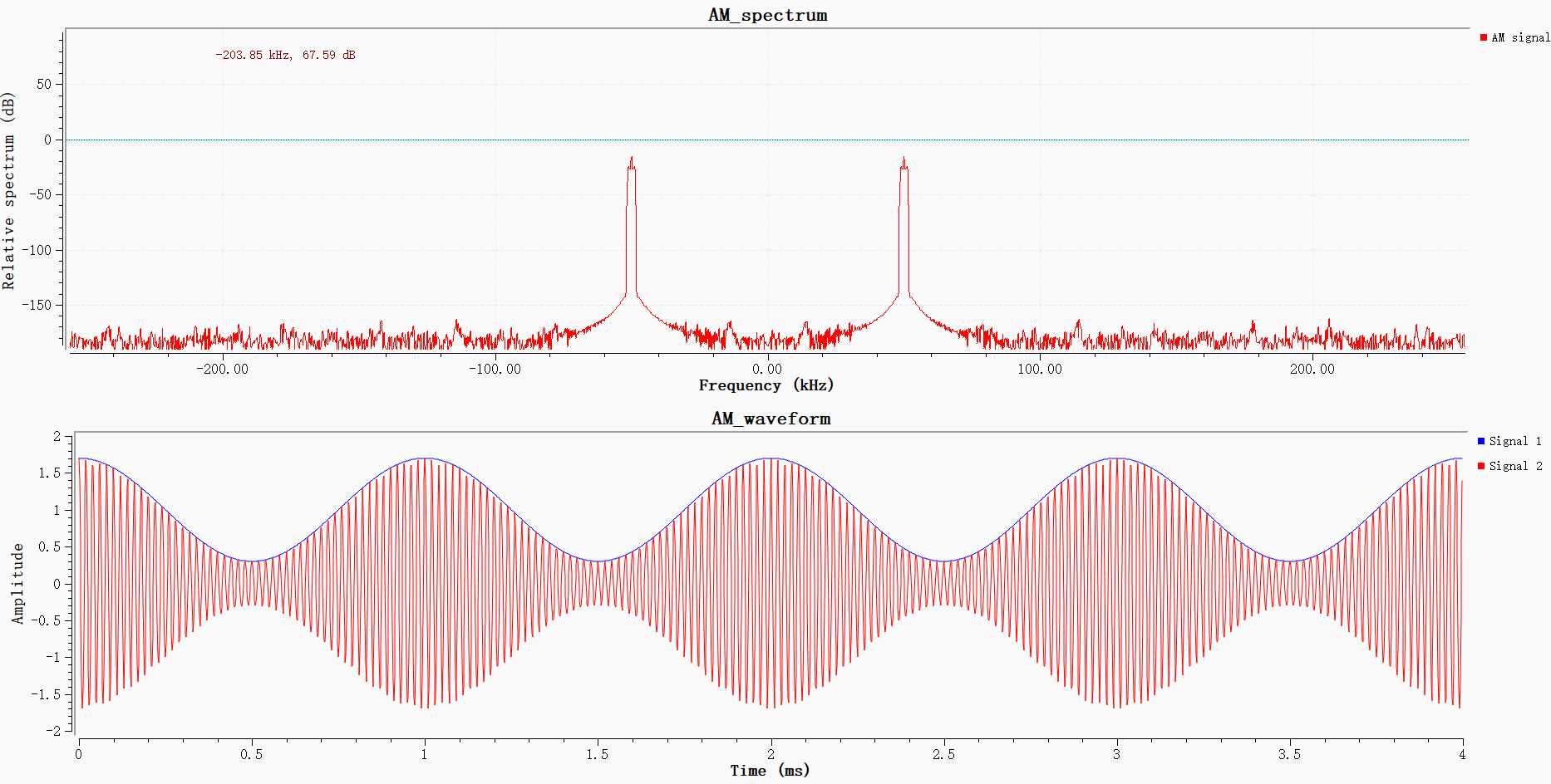
The upper plot shows the two-sided spectrum of the real-valued AM signal. Positive and negative frequencies are symmetric, so a signal cluster appears at both -50 kHz and +50 kHz. Each cluster contains the carrier, upper sideband, and lower sideband. Because the sidebands are only 1 kHz from the carrier, the three spectral lines are close together and appear as one cluster.
In the lower time-domain plot, blue shows the original low-frequency signal to be transmitted, and red shows the high-frequency AM signal. The outline of the red waveform follows the blue waveform, indicating that the carrier amplitude is modulated by the baseband signal without visible overmodulation distortion.
AM Transmit/Receive and Spectrum Observation
Open AM_Single_ADRV9009_Loopback.grc and connect antennas to the ADRV9009 RX1 and TX1 ports.
At the transmitter, Wav File Source reads 48 kHz audio. Amplitude scaling and a DC offset perform baseband AM modulation, followed by resampling, low-pass filtering, and digital upconversion with Rotator to a 40 kHz intermediate frequency. The signal is split: one branch goes to the spectrum display, and the other is converted to the required format and transmitted through ADRV9009 TX1. At the receiver, ADRV9009 RX1 captures the RF I/Q signal and splits it into two branches. One goes to the receive-spectrum display; the other passes through a frequency-translating FIR filter for digital downconversion, magnitude detection for AM envelope detection, then low-pass filtering, DC blocking, gain adjustment, and limiting before Audio Sink plays the demodulated audio. The spectrum displays in the flowgraph correspond to the spectrum screenshots. The complete chain performs AM modulation, RF transmission and reception, envelope detection, and audio recovery.
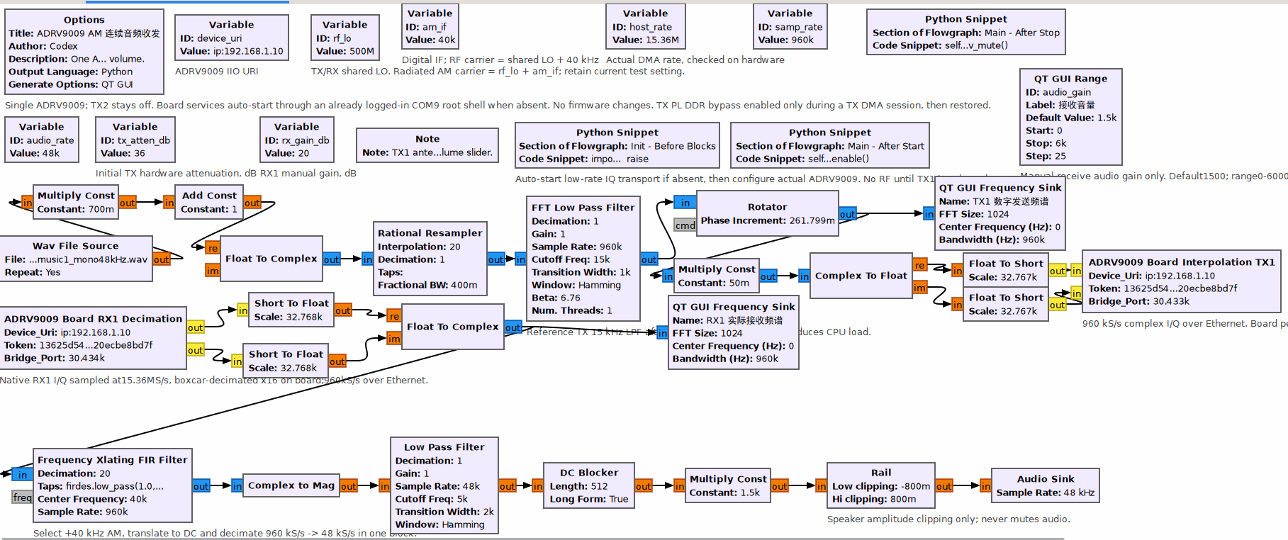
Results:
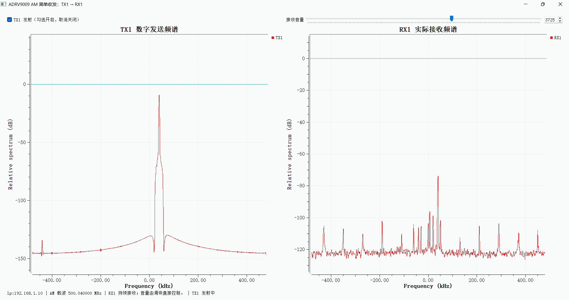
The spectrum on the left is the TX1 digital transmit baseband spectrum. It has a strong carrier at 0 kHz and symmetric AM sidebands on either side, the typical spectrum of an AM signal. The noise floor is steady and spurious components are sparse, indicating that baseband AM generation is working. The spectrum on the right is the signal actually received by RX1. It contains the corresponding AM signal cluster, confirming that the receive chain can receive the AM RF signal transmitted by TX1.
OOK (ASK) Modulation/Demodulation and Packet-Based File Transfer Simulation
OOK (ASK) Modulation Simulation and Time/Frequency Observation
1. Open ASK_mod.grc and run it to observe the carrier's time-domain waveform as it switches with the bits, along with its spectrum.
The flowgraph contains two signal sources. A cosine source generates a 10 kHz carrier, and a square-wave source generates a 1 kHz baseband signal. The signals are multiplied to perform OOK (on-off keying) modulation. Throttle controls the data rate. The modulated signal is then split into two branches connected to QT GUI time-domain and frequency-domain displays to observe the OOK waveform and spectrum.
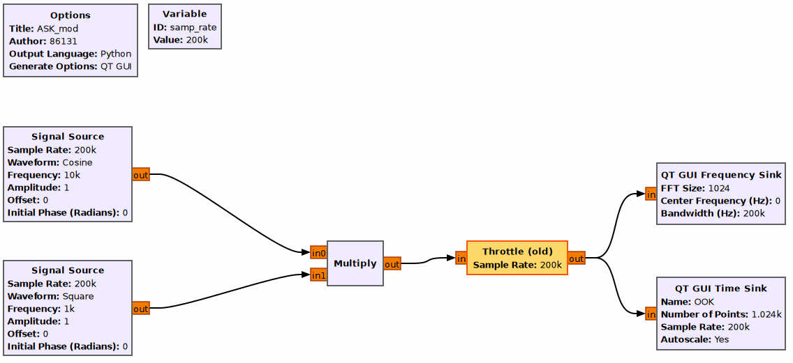
Results:
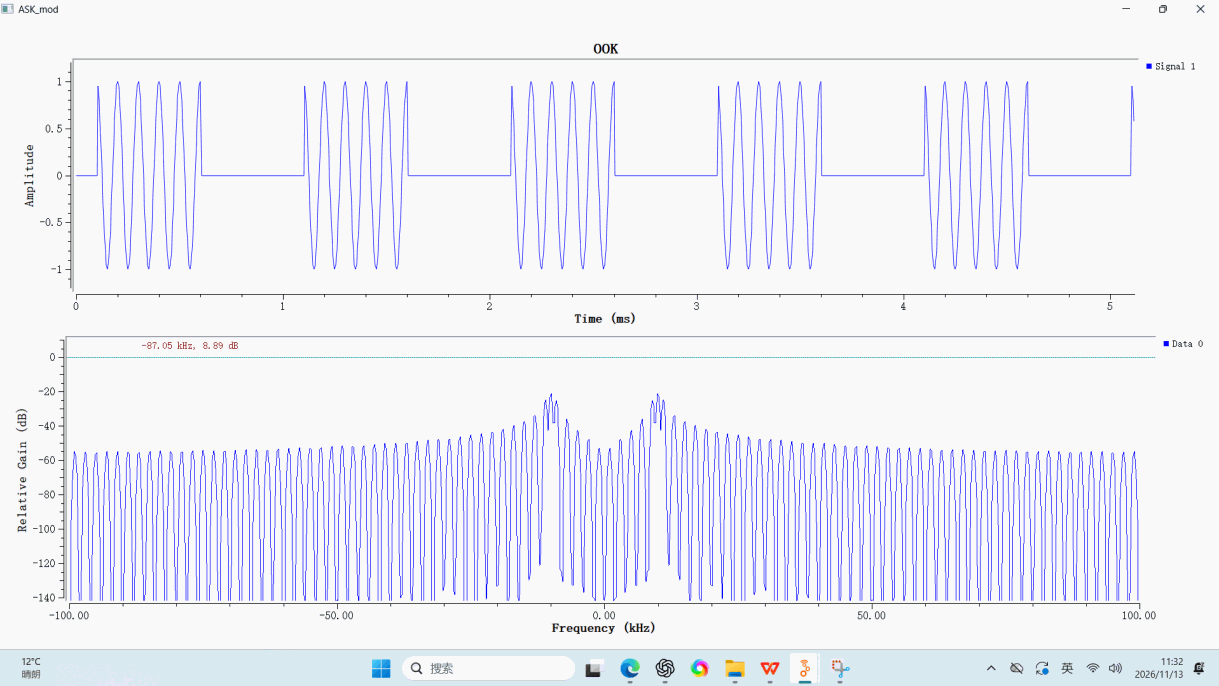
The upper plot is the time-domain waveform, with time in milliseconds on the horizontal axis and signal amplitude on the vertical axis. It shows an OOK-modulated signal, a form of ASK (amplitude-shift keying). The baseband is a 1 kHz square wave and the carrier is a 10 kHz cosine wave. When the square wave is high, the high-frequency carrier is present, representing bit 1. When it is low, the signal amplitude is zero and the carrier is off, representing bit 0. The waveform clearly shows the carrier switching on and off with each symbol, with no obvious distortion.
The lower plot is the OOK spectrum, with frequency in kHz on the horizontal axis and relative signal gain on the vertical axis. Because the signal is real-valued, its spectrum is symmetric about zero. A main spectral lobe appears at each carrier frequency, ±10 kHz. The square-wave modulating signal contains many harmonics, so continuous side lobes appear on both sides of the carrier, forming a band-shaped spectrum. In effect, the baseband square-wave spectrum is shifted to the carrier frequency, as expected for OOK modulation. The simulation result is correct.
2. Open ASK\ASK_mod_demod.grc.
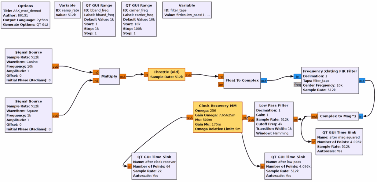
At the transmitter, a 10 kHz cosine carrier and a 1 kHz square-wave baseband signal are multiplied to generate an OOK-modulated signal. Throttle controls the rate, then Float To Complex converts the signal to complex form for a frequency-translating FIR filter. The downconverted output goes to Complex to Mag^2 for magnitude-squared detection. The detected signal is split into two branches: one displays the magnitude-squared waveform, and the other goes through a low-pass filter to remove high-frequency components. The low-pass output is split again: one branch displays the filtered waveform, while the other goes to MM Clock Recovery for symbol synchronization and recovery of the original baseband symbols, which are displayed in the time domain.
Results:
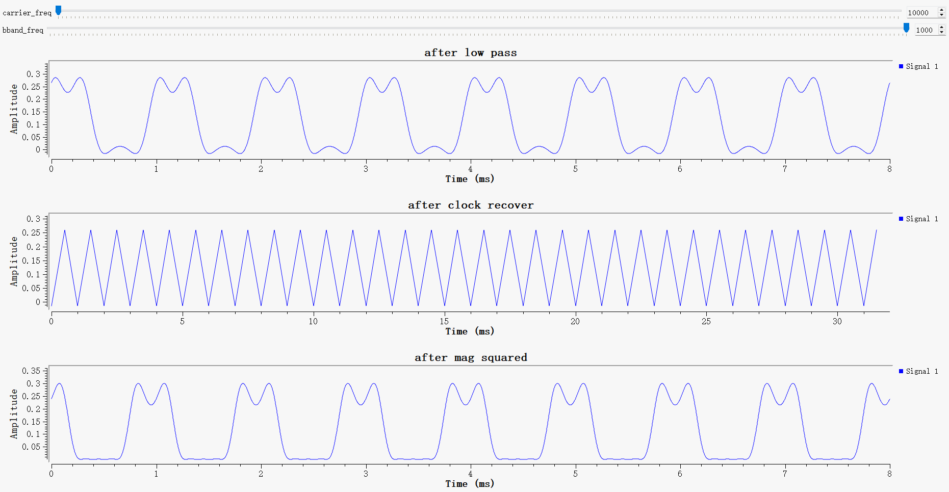
The upper waveform is the low-pass-filtered signal, with time in milliseconds on the horizontal axis and signal amplitude on the vertical axis. Magnitude-squared detection and low-pass filtering remove the carrier's high-frequency component, leaving a baseband envelope that matches the original square wave. The envelope follows the transmitter's square wave, and the high-frequency carrier ripple is removed.
The middle waveform is the clock-recovery output, with time in milliseconds on the horizontal axis and signal amplitude on the vertical axis. MM Clock Recovery performs symbol synchronization and outputs a periodic sawtooth timing signal used to align the symbol sampling instants.
The lower waveform is the signal after magnitude-squared detection, with time in milliseconds on the horizontal axis and signal amplitude on the vertical axis. Magnitude-squared detection extracts the OOK amplitude envelope and preserves the baseband square-wave shape, with a small amount of carrier ripple remaining. The low-pass filter smooths it. The demodulation chain successfully extracts the baseband envelope carried by the OOK signal and performs envelope detection and symbol-timing synchronization. The waveform matches the theoretical behavior of non-coherent OOK demodulation, so the simulation is working correctly.
OOK File Transfer Simulation with Frame Synchronization
Open ASK_file.grc, run it for at least 5 seconds, and then stop it normally.
The transmitter reads a text file and packages the data with Stream to Tagged Stream. Protocol Formatter adds the frame header, and Repeat performs interpolation for symbol shaping. The binary bit sequence is modulated onto a 10 kHz OOK carrier. One branch goes to a time-domain display for real-time observation of the modulated waveform. The receive branch uses envelope detection: it takes the absolute value of the OOK signal, then an integrate-and-dump block averages the samples in each symbol to obtain the symbol envelope. A threshold detector recovers the bits, and an access-code correlator performs frame detection and synchronization. The synchronized bitstream is reassembled into bytes and written to the output text file.
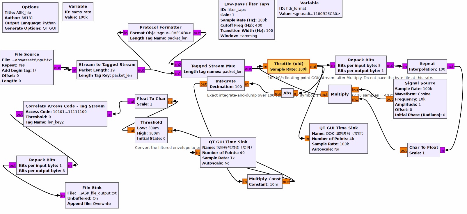
Results:
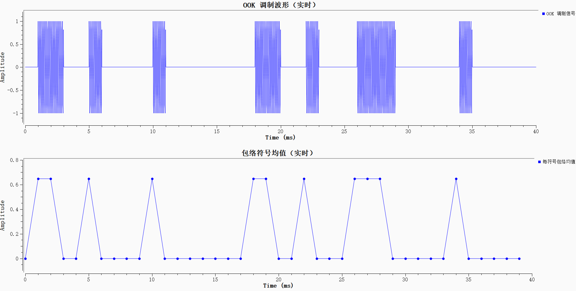
The upper plot is the OOK-modulated signal in the time domain. The carrier frequency is 10 kHz; bit 1 turns the carrier on, and bit 0 turns it off, as expected for on-off keying. The lower plot shows the symbol-envelope averages after integrate-and-dump processing. Envelope detection and averaging over each symbol period remove the carrier's high-frequency ripple and map the transmitted bits to two distinct envelope levels. This confirms that integrate-and-dump non-coherent OOK demodulation is effective.
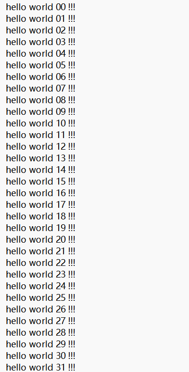
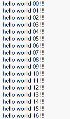
Stop the flowgraph and open ASK_file_output.txt in the outputs folder. Check that the original text, including “hello world 00 !!!”, was recovered successfully.
BPSK Synchronization and Text Transmission Experiments
BPSK Baseband Modulation Simulation and Signal Characteristics
1. Open BPSK_mod.grc.
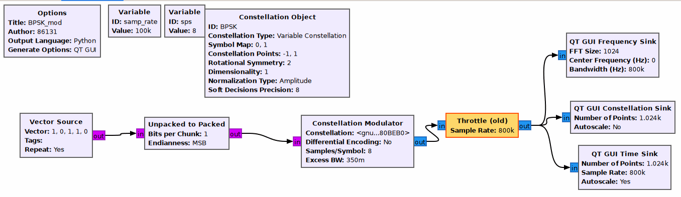
Vector Source repeatedly outputs the bit sequence [1, 0, 1, 1, 0] as the baseband data source. Unpacked to Packed repacks the individual bits into the format required by the modulator. Constellation Object defines the BPSK constellation, with points at -1 and +1 on the real axis of the complex plane, representing two symbols whose phases differ by 180°. Constellation Modulator maps bits to symbols and applies root-raised-cosine pulse shaping. Differential encoding is disabled; the signal is oversampled by 8 samples per symbol, with a roll-off factor of 0.35. Throttle controls the simulation data rate. The modulated signal is sent to three QT GUI displays for the time-domain waveform, spectrum, and constellation.
Results:
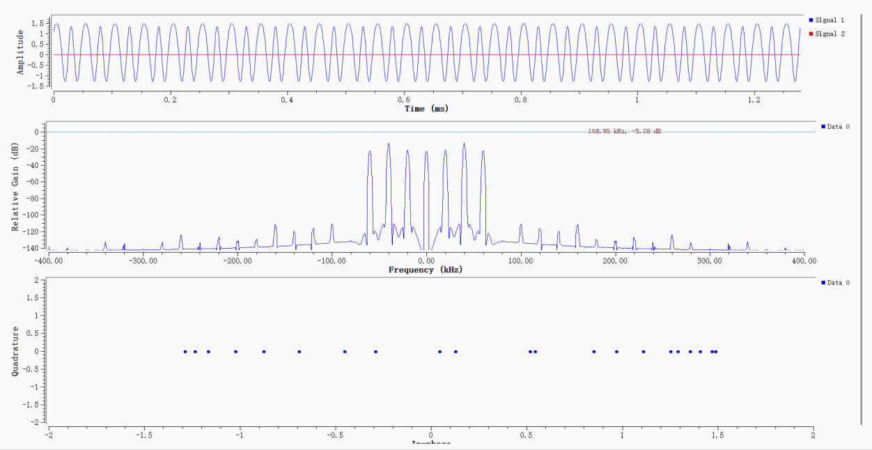
The simulation window has three plots: time domain, frequency domain, and constellation. The upper time-domain plot shows the BPSK baseband signal after root-raised-cosine shaping, alternating between positive and negative levels. The middle plot shows the shaped BPSK spectrum, with its main lobe concentrated near zero frequency and clearly attenuated side lobes, as expected from root-raised-cosine filtering. In the lower constellation plot, the signal points converge on +1 and -1 on the real axis, with little spread. This indicates that BPSK symbol mapping and pulse shaping are working well.
File-Based BPSK Modulation/Demodulation and Frame Synchronization
Open BPSK\BPSK_file.grc.
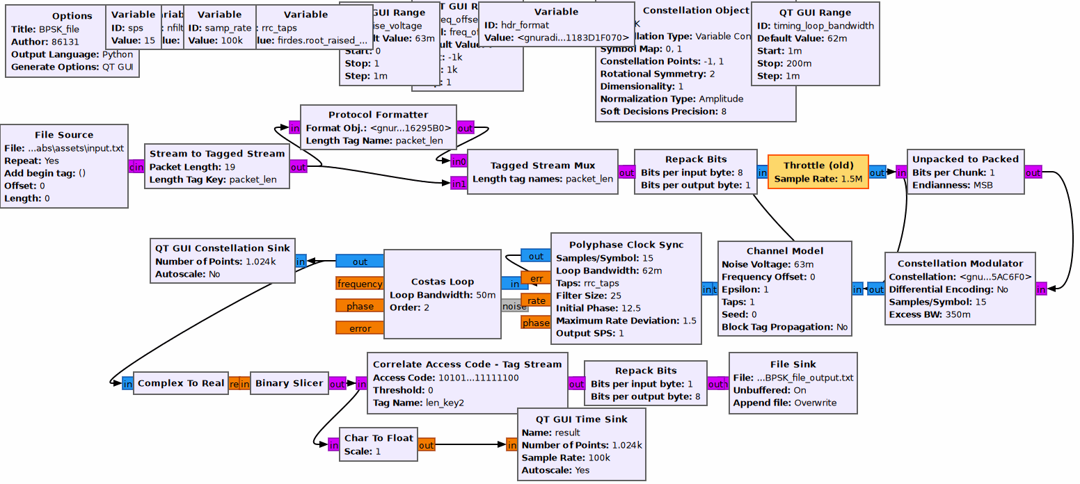
File Source reads the bit data in input.txt. Stream to Tagged Stream adds packet-length tags, Protocol Formatter adds a frame header, and Tagged Stream Mux assembles the frame. After Repack Bits, Throttle, and Unpacked to Packed perform the required data-format conversions, Constellation Modulator applies BPSK mapping with differential encoding disabled, 15 samples per symbol, and a 0.35 roll-off factor, then performs root-raised-cosine pulse shaping. Channel Model adds Gaussian noise. Polyphase Clock Sync and Costas Loop then perform timing and carrier synchronization. The synchronized signal is split into two branches: one goes to QT GUI Constellation Sink for constellation display; the other passes through Complex To Real and Binary Slicer for decisions, then Correlate Access Code - Tag Stream for frame synchronization. Repack Bits reassembles the bytes, and File Sink saves the demodulated output bits to BPSK_file_output.txt. A QT GUI Time Sink also displays the recovered baseband waveform.
Results:
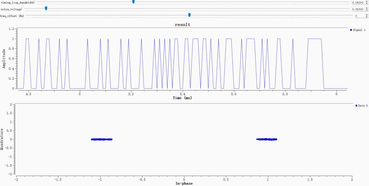
The upper time-domain plot shows the recovered binary baseband signal, with high and low levels clearly distinguishing bits 0 and 1. In the lower constellation plot, points lie near ±1 on the real axis. They are somewhat spread out compared with the noise-free simulation because Gaussian noise was added to the channel, but the two clusters remain distinct. The timing synchronizer and Costas carrier loop have converged, allowing the system to demodulate the BPSK signal, acquire frames, and recover the bits correctly.
Run the flowgraph for about 5 seconds, stop it, and inspect the text content and record order in outputs\BPSK_file_output.txt. Differential encoding at the transmitter and differential decoding at the receiver must be configured as a pair.
FM Modulation and Audio Recovery Experiments
Generating and Observing a Wideband FM Signal
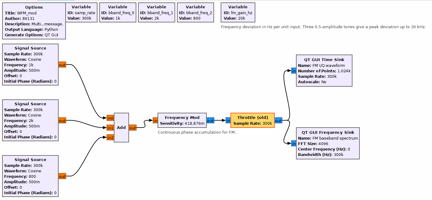
Open WFM_mod.grc. Three Signal Source blocks generate 800 Hz, 1 kHz, and 2 kHz tones. Add combines them into a composite baseband modulating signal, which is sent to Frequency Mod for FM modulation with a sensitivity of 418.879m and continuous phase accumulation. Throttle controls the simulation data rate. The complex FM signal is split into two branches and sent to QT GUI Time Sink and QT GUI Frequency Sink to observe the I/Q time-domain waveforms and the FM baseband spectrum.
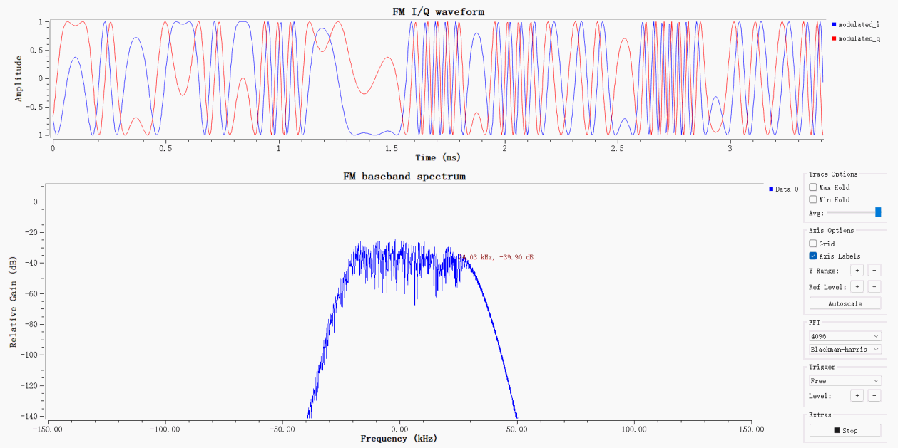
The upper time-domain plot shows the I and Q waveforms after FM modulation. The signal amplitude remains constant while its instantaneous frequency varies with the composite baseband signal, as expected for FM. The lower plot shows the wideband FM baseband spectrum, which has a bell-shaped distribution with energy concentrated around the carrier. Its bandwidth is determined by the maximum frequency deviation and the modulating-signal bandwidth, consistent with wideband FM theory.
Single-Device FM Audio Loopback
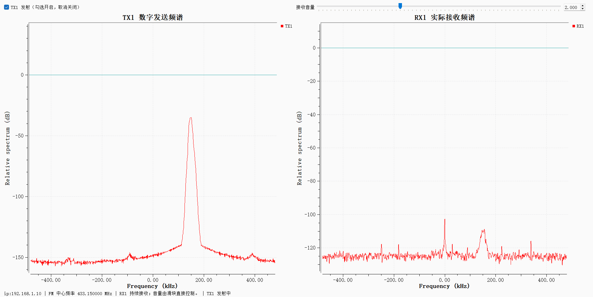
Open WFM_tx_rx_ADRV9009.grc. Wav File Source reads a 48 kHz audio file, which passes through two interpolating low-pass filters and then Frequency Mod for wideband FM modulation. After frequency-offset shifting and amplitude scaling, the signal is transmitted over the ADRV9009 transmit channel. On reception, the ADRV9009 captures the RF signal; after downconversion and decimation filtering, complex-conjugate multiplication performs FM demodulation. The signal then passes through low-pass filtering, DC removal, and amplitude limiting before Audio Sink plays the recovered audio. The TX1 and RX1 spectrum displays show the transmit baseband spectrum and the received RF spectrum in real time.
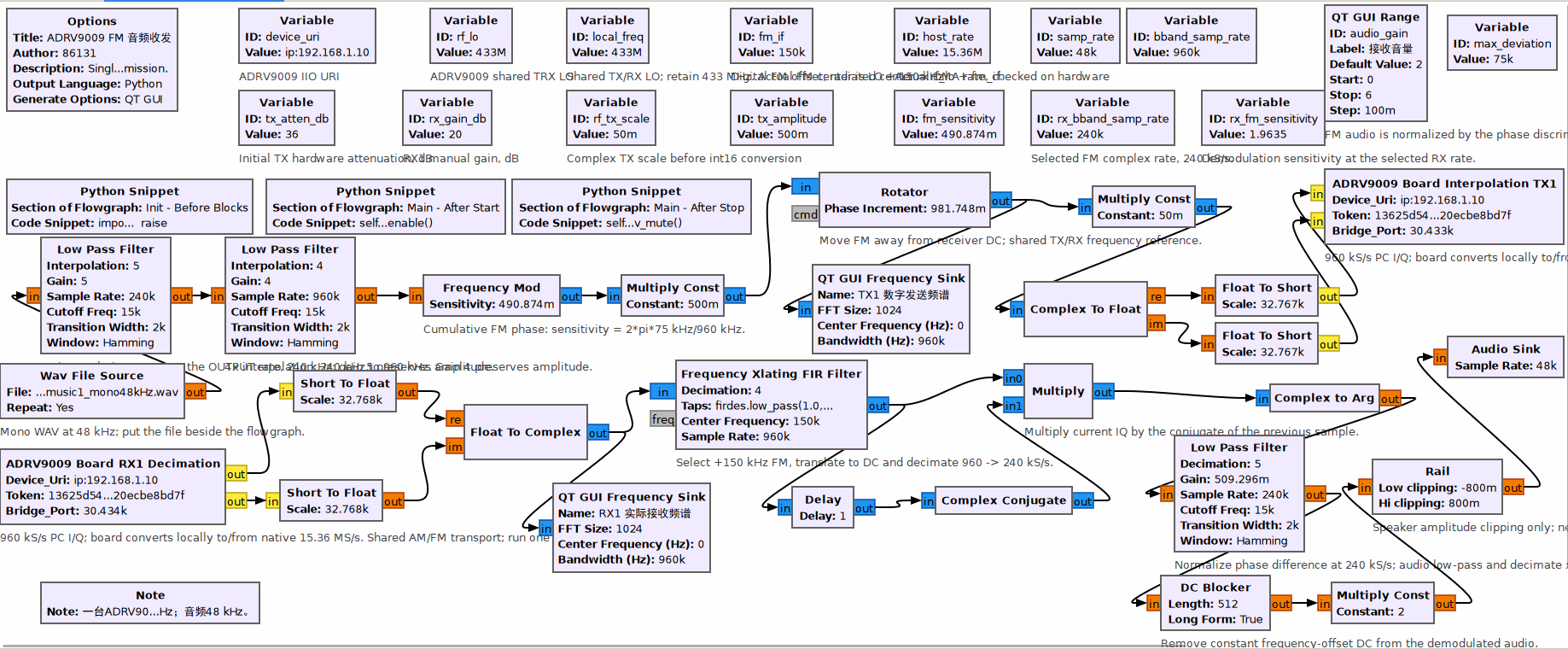
The spectrum on the left shows the wideband FM signal transmitted by TX1, with concentrated energy and a typical FM spectrum. The spectrum on the right shows the RF signal received by ADRV9009 RX1. A noise floor is present, but the carrier and sideband structure are clear. The hardware transmit/receive chain is operating and can carry and demodulate an FM audio signal for playback.
QPSK Synchronization and Text Transmission Experiments
Synchronized QPSK File-Transfer Simulation with Differential Encoding
Open QPSK_file.grc. File Source reads the text in input.txt, which is framed and bit-reordered before being sent to the QPSK constellation modulator with differential encoding enabled. The modulated signal passes through a channel model that adds noise and frequency offset. The receiver performs polyphase clock synchronization, Costas-loop carrier synchronization, constellation demodulation, and differential decoding. A correlation-based synchronizer then detects the frame header, and the bits are reassembled. The recovered data is written to QPSK_file_output.txt. QT GUI Constellation Sink and QT GUI Time Sink display the constellation and recovered bit waveform.
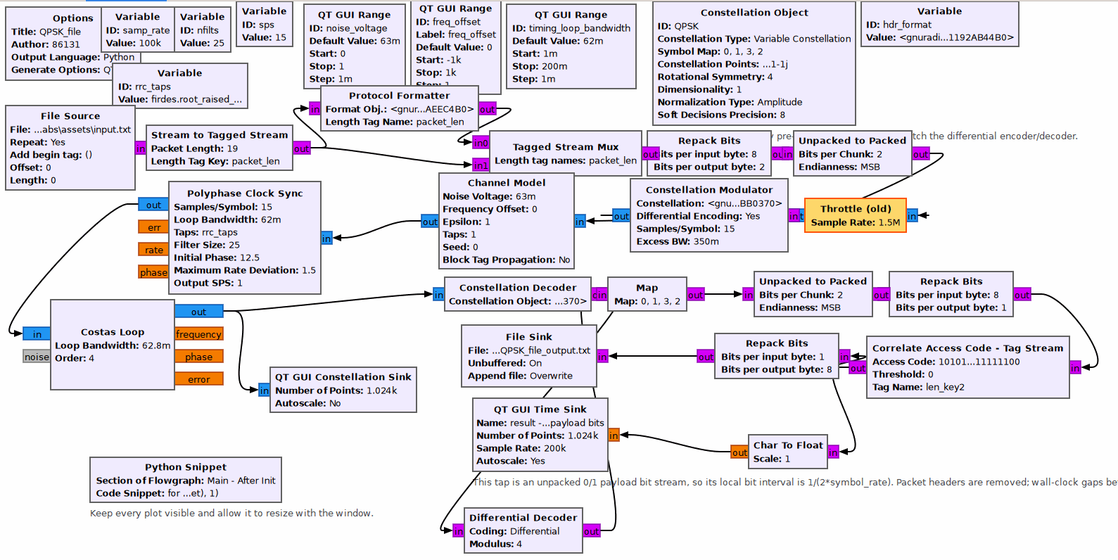
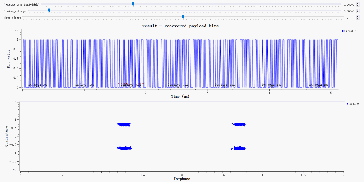
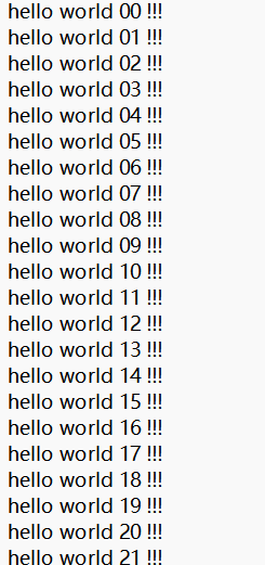
The upper time-domain plot shows the recovered payload bitstream, and the frame markers are present. The lower constellation plot shows the four QPSK points; the synchronization loops have converged and the points are distinct. The system can transmit text using QPSK and restore it to a file under noise and frequency offset. Open outputs\QPSK_file_output.txt.
IIO Oscilloscope Testing
Open IIO Oscilloscope. In the connection window, select Manual, enter ip:192.168.1.10, click Refresh, verify the ADRV9009 device list, and click Connect.
Capturing the RX Spectrum Baseline
Switch to the ADRV9009 Controls page and configure the following parameters:
RF local oscillator: 5000 MHz
RX1: Set the mode to manual, set gain to 20 dB, and clear RX1 Powerdown.
TX1 and TX2: Set TX1 attenuation to 36 dB and select Powerdown Enable so the transmit path is initially off.
TX1 DDS: Select One CW Tone mode, set frequency to 0.5 MHz, Scale to -26 dBFS, and phase to 90°.
TX2 DDS: Set to Disable.
Scroll down to FPGA Settings and set the Sampling Rate for both the transmit and receive DMA buffers to 15360000.
In the main window, select File → New Plot to create a capture window. Set Plot Type to Frequency Domain. Select axi-adrv9009-rx-hpc and check only voltage0_i and voltage0_q. Configure the FFT parameters: FFT Size = 16384, window = Hanning, Window Correction enabled, Average = 16, and PWR Offset = 0. Leave Auto scale and Show grid enabled. Click Capture/Stop on the toolbar to start continuous capture. Right-click the plot area and open Peak Markers.
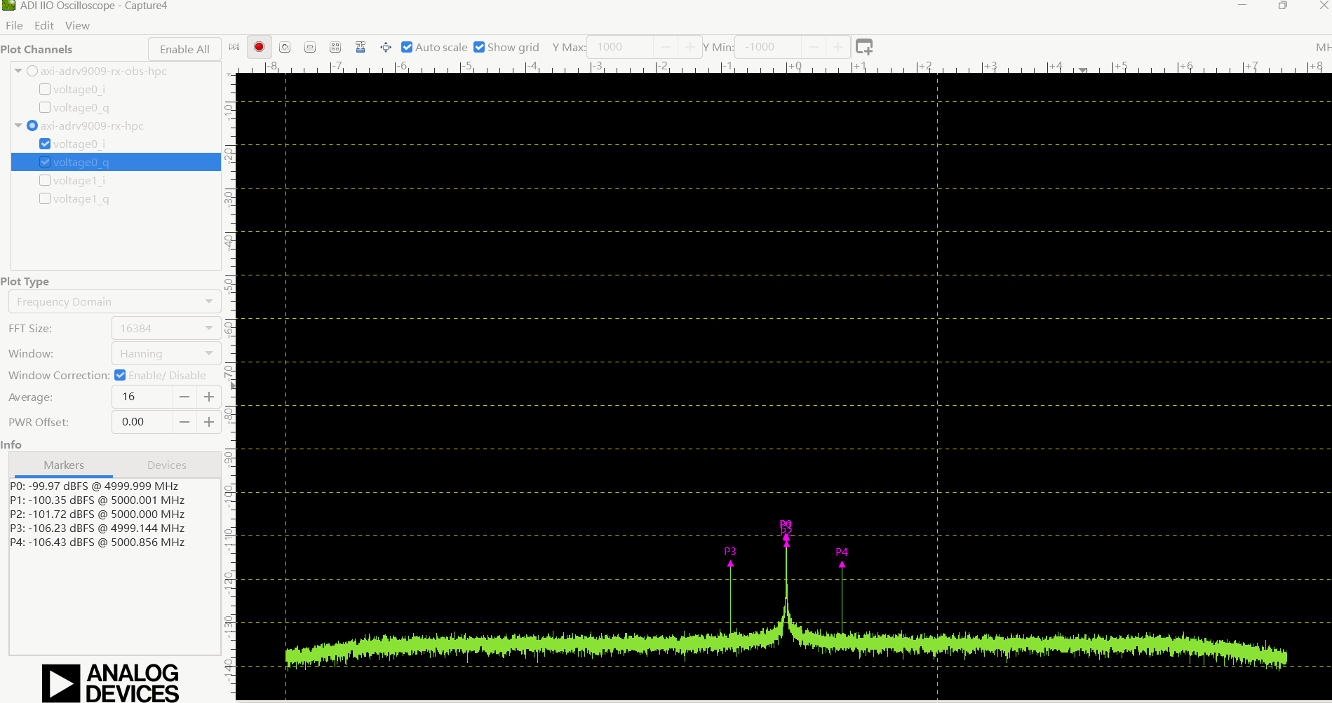
After configuring the parameters and starting capture, the RX1 spectrum window shows a continuously varying green noise floor across the baseband span of -7.68 to +7.68 MHz. A prominent center spike appears at zero frequency. Peak Markers reads close to 5000 MHz at about -100 dBFS, with a few narrowband inherent spurs beside the center peak. TX1 and TX2 are both powered down, so although the DDS is configured for a 0.5 MHz tone, no target test peak appears at +0.5 MHz to the right of zero. This baseline is as expected and provides a clean receive-background reference.
Observing a Received Single Tone
Keep TX2 off and clear Powerdown Enable for TX1 only, then return to the Capture window. Check for a narrowband peak near +0.5 MHz to the right of zero and read its frequency in Markers.
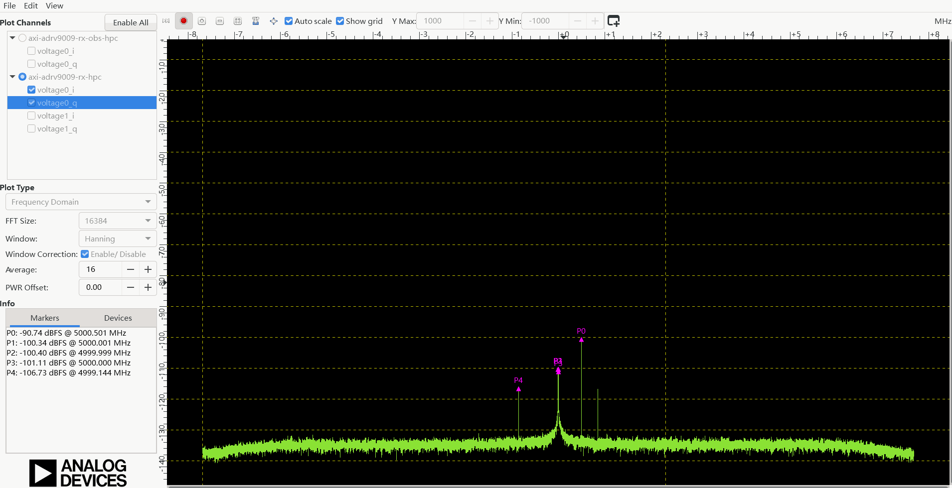
After TX1 is enabled, a clear narrowband spike appears near +0.5 MHz to the right of zero, above the surrounding noise floor. In the screenshot, marker P0 reads 5000.501 MHz, consistent with the 5000 MHz local oscillator plus the 0.500632 MHz DDS output. The spectrum's horizontal axis shows baseband offset relative to the receive center, while Peak Marker shows the absolute RF frequency including the local oscillator. Thus, +0.5 MHz baseband offset and 5000.501 MHz absolute RF frequency refer to the same test signal. The peak appears when TX is enabled, confirming that the transmit and receive paths are working.
Verifying DDS Frequency Tracking at 1 MHz
Keep the local oscillator, gain, transmit attenuation, and amplitude unchanged. Change TX1 DDS Frequency from 0.5 MHz to 1 MHz, apply the setting, return to the Capture window, and check whether the peak moves from about +0.5 MHz to about +1 MHz.
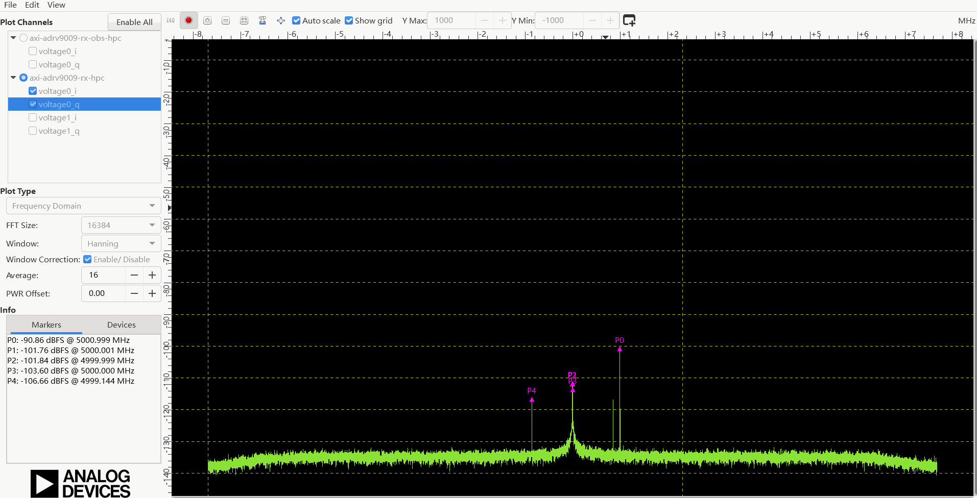
After the DDS frequency is changed, the target narrowband spike moves farther to the right of zero, and the test peak is no longer present at +0.5 MHz. The hardware reports a DDS frequency of 999390 Hz, while the software marker reads an RF frequency of about 5000.999 MHz, corresponding to a baseband offset of about +1 MHz, as expected.
The test peak moves with the DDS setting: the old test tone disappears and a corresponding spike appears at the new frequency. This confirms that the peak is generated by the local DDS and that the transmit output frequency reliably follows the DDS configuration.